Chapter 4 Model establishment via GSClassifier
4.1 About
Sometimes, researchers might have their gene signatures and know how many subtypes they want to call before (based on some knowledge). Gratifyingly, comprehensive functions were also provided in GSClassifier. In this section, we would show how to build a GSClassifier model like PADi.
4.2 Data preparation
Load packages:
Load data:
# The test data is only for the demonstration of the modeling
testData <- readRDS(system.file("extdata", "testData.rds", package = "GSClassifier"))
expr <- testData$PanSTAD_expr_part
design <- testData$PanSTAD_phenotype_part
Select training and testing cohorts across different platforms and PAD subtypes from PAD function:
modelInfo <- modelData(
    design,
    id.col = "ID",
    variable = c("platform", "PAD_subtype"),
    Prop = 0.7,
    seed = 145
  )
Check the result modelInfo:
Explore the training cohort:
head(modelInfo$Data$Train)
#                    ID  Dataset PAD_subtype PIAM_subtype PIDG_subtype platform
# GSM1606527 GSM1606527 GSE65801       PAD-I         high         high GPL14550
# GSM1606553 GSM1606553 GSE65801       PAD-I         high         high GPL14550
# GSM1606517 GSM1606517 GSE65801       PAD-I         high         high GPL14550
# GSM1606503 GSM1606503 GSE65801       PAD-I         high         high GPL14550
# GSM1606509 GSM1606509 GSE65801       PAD-I         high         high GPL14550
# GSM1606551 GSM1606551 GSE65801       PAD-I         high         high GPL14550
Explore the internal validation cohort:
head(modelInfo$Data$Valid)
#                    ID  Dataset PAD_subtype PIAM_subtype PIDG_subtype platform
# GSM2235559 GSM2235559 GSE84437      PAD-II         high          low  GPL6947
# GSM2235564 GSM2235564 GSE84437      PAD-IV          low          low  GPL6947
# GSM2235566 GSM2235566 GSE84437      PAD-IV          low          low  GPL6947
# GSM2235567 GSM2235567 GSE84437      PAD-IV          low          low  GPL6947
# GSM2235568 GSM2235568 GSE84437      PAD-IV          low          low  GPL6947
# GSM2235571 GSM2235571 GSE84437      PAD-IV          low          low  GPL6947
Get training data Xs and Ys:
# Training data
Xs <- expr[,modelInfo$Data$Train$ID]
y <- modelInfo$Data$Train
y <- y[colnames(Xs),]
Ys <- ifelse(y$PAD_subtype == 'PAD-I',1,ifelse(y$PAD_subtype == 'PAD-II',2,ifelse(y$PAD_subtype == 'PAD-III',3,ifelse(y$PAD_subtype == 'PAD-IV',4,NA)))); table(Ys)/length(Ys)
# Ys
#         1         2         3         4
# 0.1010169 0.2474576 0.1694915 0.4820339
Get the number of subtype:
Also, you can take a look at the validation data:
# Validating data
Xs_valid <- expr[,modelInfo$Data$Valid$ID]
y <- modelInfo$Data$Valid
y <- y[colnames(Xs_valid),]
Ys_valid <- ifelse(y$PAD_subtype == 'PAD-I',1,ifelse(y$PAD_subtype == 'PAD-II',2,ifelse(y$PAD_subtype == 'PAD-III',3,ifelse(y$PAD_subtype == 'PAD-IV',4,NA))))
table(Ys_valid)/length(Ys_valid)
# Ys_valid
#          1          2          3          4
# 0.09609121 0.24592834 0.16612378 0.49185668
Note: When you convert your phenotype into numeric, You CANNOT USE A ZERO VALUE, which is not supported by the xGboost.
Other parameteres for modeling:
# Build 20 models
n=20

# In every model, 70% samples in the training cohort would be selected.
sampSize=0.7

# Seed for sampling
sampSeed = 2020
na.fill.seed = 2022

# A vector for approximate gene rank estimation
breakVec=c(0, 0.25, 0.5, 0.75, 1.0)

# Use 80% most variable gene & gene-pairs for modeling
ptail=0.8/2

# Automatical selection of parameters for xGboost
auto = F

if(!auto){

      # Self-defined params. Fast.
      params = list(max_depth = 10,
                    eta = 0.5,
                    nrounds = 100,
                    nthread = 10,
                    nfold=5)
      caret.seed = NULL

      # No. of CPU for parallel computing. The optimized value depends on your CPU and RAM
      numCores = 4

    } else {

      # caret::train strategy by GSClassifier:::cvFitOneModel2. Time consuming
      params = NULL
      caret.seed = 105

      # Self-defined. For this exmaple training grid, there are 2×1×1×3×2×1×2=24 grids. Make sure that you have a computer with a powerfull CPU.
      grid = expand.grid(
        nrounds = c(100, 200),
        colsample_bytree = 1,
        min_child_weight = 1,
        eta = c(0.01, 0.1, 0.3),
        gamma = c(0.5, 0.3),
        subsample = 0.7,
        max_depth = c(5,8)
      )

      # If you don't know how to set, just use the same number of your subtypes
      numCores = 4
    }
Finaly, you have to provide your gene sets as a list object:
geneSet = <Your gene sets>
Let’s take PAD as an example:
PAD <- readRDS(system.file("extdata", "PAD.train_20220916.rds", package = "GSClassifier"))
geneSet <- PAD$geneSet
print(geneSet)
# $PIAM
#  [1] "ENSG00000122122" "ENSG00000117091" "ENSG00000163219" "ENSG00000136167"
#  [5] "ENSG00000005844" "ENSG00000123338" "ENSG00000102879" "ENSG00000010671"
#  [9] "ENSG00000185862" "ENSG00000104814" "ENSG00000134516" "ENSG00000100055"
# [13] "ENSG00000082074" "ENSG00000113263" "ENSG00000153283" "ENSG00000198821"
# [17] "ENSG00000185811" "ENSG00000117090" "ENSG00000171608"
#
# $PIDG
#  [1] "ENSG00000116667" "ENSG00000107771" "ENSG00000196782" "ENSG00000271447"
#  [5] "ENSG00000173517" "ENSG00000134686" "ENSG00000100614" "ENSG00000134247"
#  [9] "ENSG00000109686" "ENSG00000197321" "ENSG00000179981" "ENSG00000187189"
# [13] "ENSG00000140836"
4.3 Fitting models
4.3.1 GSClassifier model training
Just fit the model like:
if(!auto){

  # Self-defined

  system.time(
    res <- fitEnsembleModel(Xs,
                            Ys,
                            geneSet = geneSet,
                            na.fill.method = c('quantile','rpart',NULL)[1],
                            na.fill.seed = na.fill.seed,
                            n = n,
                            sampSize = sampSize,
                            sampSeed = sampSeed ,
                            breakVec = breakVec,
                            params = params,
                            ptail = ptail,
                            caret.grid = NULL,
                            caret.seed =  caret.seed,
                            verbose = verbose,
                            numCores = numCores)
  )

  # user   system  elapsed
  # 0.08s  0.18s   92.70s

} else {

  # caret::train-defined and time-consuming
  system.time(
    res <- fitEnsembleModel(Xs,
                            Ys,
                            geneSet = geneSet,
                            na.fill.method = c('quantile','rpart',NULL)[1],
                            na.fill.seed = na.fill.seed,
                            n = n,
                            sampSize = sampSize,
                            sampSeed = sampSeed ,
                            breakVec = breakVec,
                            params = NULL,  # This must be NULL
                            ptail = ptail,
                            caret.grid = grid,
                            caret.seed =  caret.seed,
                            verbose = verbose,
                            numCores = numCores)
  )

  # user   system   elapsed
  # 1.10s  2.60s    2311.55s
}

# Remind me with a music when the process completed
mymusic()
You should save it for convenience:
saveRDS(res,'<your path>/train_ens.rds')Although an auto-parameter strategy (hyperparameter tuning) was provided inGSClassifier, it’s unknown whether this method could significantly improve your model performance. You can just try. It’s not a prior recommendation. Generally, setting auto=F in this script could be more cost-effective. Empirically, the speed of caret::train depends on the single-core performance of the CPU instead of the core number.
4.3.2 Scaller for the best call
Next, we model the scaller for the training cohort, which would be used for BestCall based on the probability matrix in callEnsemble series. Here, scaller=NULL would cause an NA value of BestCall col. It’s not a big deal, because the probability matrix is the information we need.
# Time-consuming modeling
resTrain <- parCallEnsemble(X = Xs,
                            ens = res$Model,
                            geneAnnotation = res$geneAnnotation,
                            geneSet = geneSet,
                            scaller = NULL,
                            geneids = "ensembl",
                            subtype = NULL,
                            numCores = numCores)

# xgboost via best interation
library(xgboost)
dtrain <- xgb.DMatrix(as.matrix(resTrain[4:(3 + nSubtype)]), label = Ys-1)

cvRes <- xgb.cv(data = dtrain,
                nrounds=100,
                nthread=10,
                nfold=5,
                max_depth=5,
                eta=0.5,
                early_stopping_rounds=100,
                num_class = 4,
                objective = "multi:softmax")

# xgboost via best interation
bst <- xgboost(data = dtrain,
               max_depth=5,
               eta=0.5,
               nrounds = cvRes$best_iteration,
               nthread=10,
               num_class = 4,
               objective = "multi:softmax")
Ys_pred <- predict(bst, as.matrix(resTrain[4:7])) + 1
mean(Ys_pred == Ys) # Prediction rates

# Ensemble results
scaller.train <- list(
      Repeat = list(
        data = dtrain,
        max_depth=5,
        eta=0.5,
        nrounds = cvRes$best_iteration,
        nthread=10,
        num_class = 4,
        objective = "multi:softmax"
      ),
      Model = bst
    )
4.3.3 Assemble your model
For more information of geneAnnotation, you could see the Suggestions for GSClassifier model developers: Gene Annotation section for assistance.
Here we give an example:
l.train <- list()

# bootstrap models based on the training cohort
l.train[['ens']] <- res

# Scaller model
l.train[['scaller']] <- scaller.train

# a data frame contarining gene annotation for IDs convertion
l.train[['geneAnnotation']] <- <Your gene annotation>

# Your gene sets
l.train[['geneSet']] <- geneSet
Finally, save it for downstream analysis
saveRDS(l.train,'<Your path>/train.rds')About model constributions, you can go Advanced development in here or here for more information.
4.3.4 Of note
You can take a look at the PAD.train_20220916 model (PADi). You have to make your model frame similar to the PAD.train_20220916 model.
l.train <- readRDS(system.file("extdata", "PAD.train_20220916.rds", package = "GSClassifier"))
names(l.train)
# [1] "ens"            "scaller"        "geneAnnotation" "geneSet"
The time of GSClassifier modeling depends on the number of individual models (controlled by n)/called subtypes/gene signatures, automatic parameter selection, and your CPU capacity.
4.4 Calling subtypes
Supposed that you had got a GSClassifier model, next you want to use it for personalized subtype calling.
Just:
# Load your model
l <- readRDS('<Your path>/train.rds')

# subtype calling
res_i = callEnsemble(
  X,
  ens = l$ens$Model,
  geneAnnotation = l$geneAnnotation,
  geneSet = l$geneSet,
  scaller = l$scaller$Model,
  geneid = <ID type of your training data>,
  matchmode = 'fix',
  subtype = NULL,
  verbose = T
)
The usage of parCallEnsemble (for a huge amount of samples) is similar. Empirically, parCallEnsemble can not perform better than callEnsemble in a small cohort for the process of xgboost would take advantage of multiple CPU cores.
4.5 Number of SubModel
In the latest version of PADi, we trained 100 SubModels for subtype calling. We also trained some models with different training cohorts (200 models, Figure 4.1) or with different numbers (20, 50, 100, 200, 500 and 1000 for the same training cohort, Figure 4.2) of sub-models. Our results showed that the performance of these models is similar in the “Kim2018” cohort.
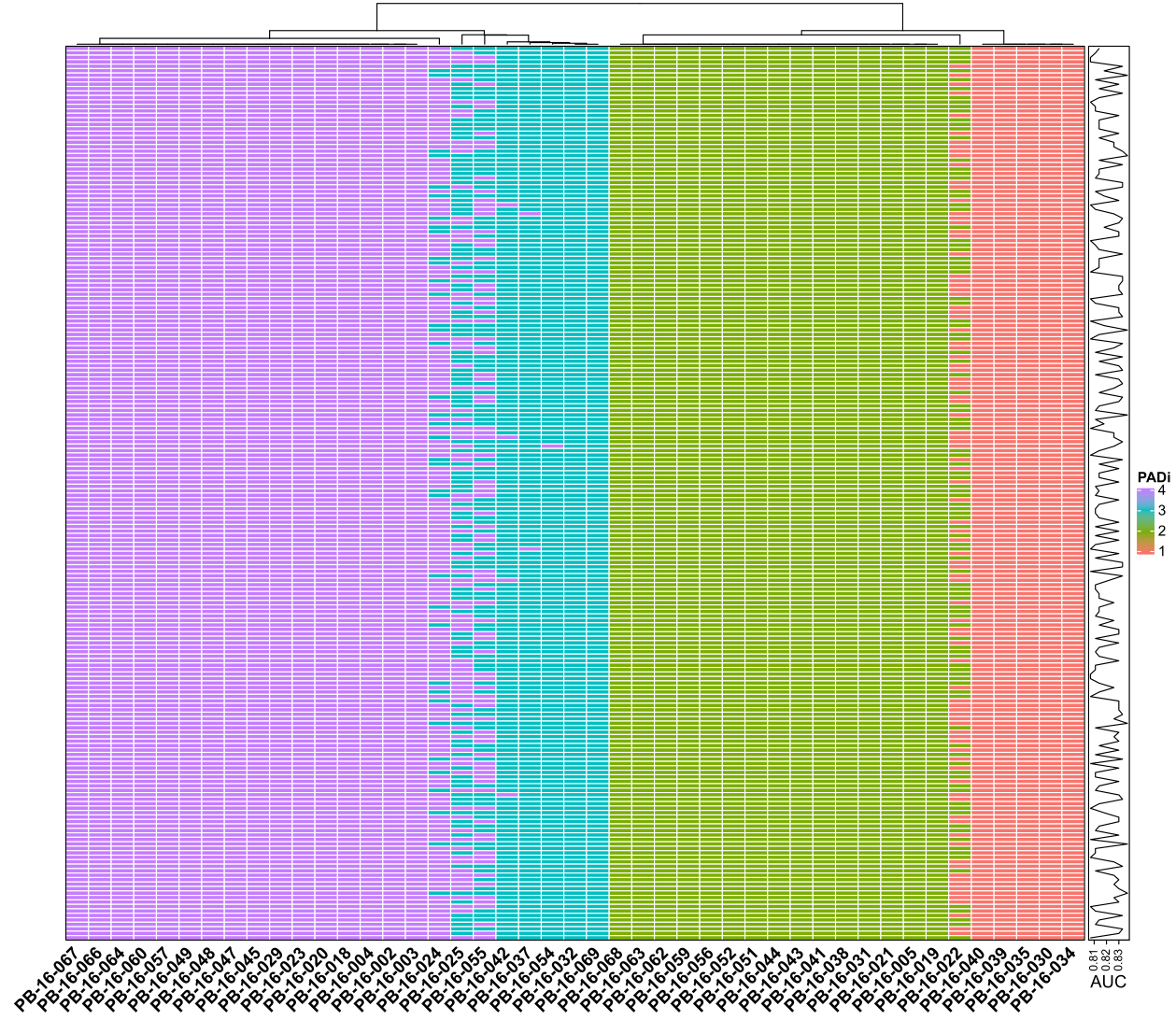
Figure 4.1: Performance of PADi models in “Kim2018” cohort with 200 different training seeds. Each row is the data of a seed. Each column is a sample from the “Kim2018” cohort.
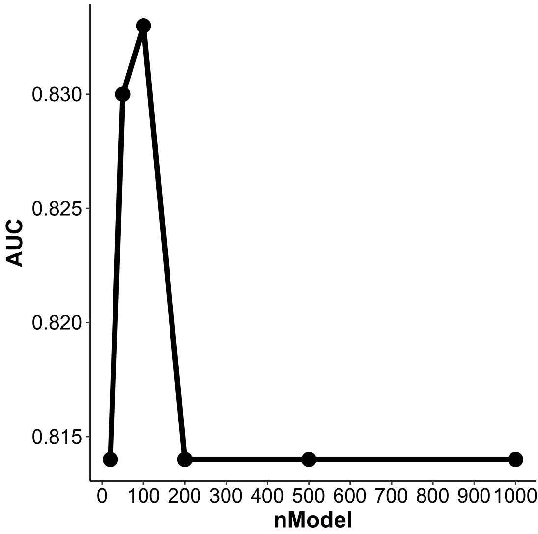
Figure 4.2: Performance of PADi models in “Kim2018” cohort with different numbers of SubModel. The x-axis is the number of SubModels, and the y-axis is the AUC of ROC analysis for ICI response prediction.
4.6 Parameters for PADi training
Here’re some key parameters about how the latest PADi (PAD.train_v20220916) was trained.
# Build 100 models
n = 100

# In every model, 70% samples in the training cohort would be selected.
sampSize = 0.7

# Seed for sampling
sampSeed = 2020
na.fill.seed = 443

# A vector for gene rank estimation
breakVec = c(0, 0.25, 0.5, 0.75, 1.0)

# Use 80% most variable gene & gene-pairs for modeling
ptail = 0.8/2

# Automatical selection of parameters for xGboost
# self-defined params. Fast.
params = list(max_depth = 10,
              eta = 0.5,
              nrounds = 100,
              nthread = 10,
              nfold=5)
caret.seed = NULL
Enjoy GSClassifier!